# load packages
library(tidyverse) # for data manipulation and visualization
library(RColorBrewer) # for color palettes
library(patchwork) # for combining plots
library(pracma) # for calculating the area of a polygon2 ggplot2“银河系”等高线
ggplot2版本的“银河系”,并计算特定等高线的面积
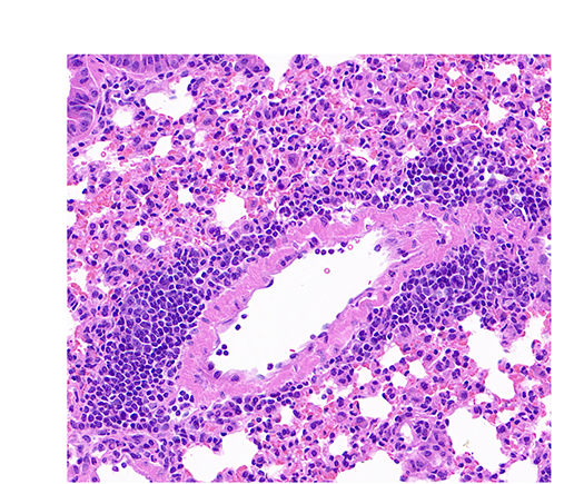
在2025-07-29日,我们展示过H&E起源版本的“银河系”(QuPath:“银河系”起源于H&E),在2025-08-12,我们通过R的ggplot2来展示该“银河系”(R:ggplot2等高线图版本的“银河系”)。
这次,我们进一步计算特定等高线的面积。
1. Load packages and read data/加载包和读取数据
加载包。
读取数据。
# read the table
txt_file <- "raw_data/2025-08-12_QuPath_InstanSeg.txt" # specify the path to the text file
df <- txt_file |> read_delim(delim = "\t", col_names = TRUE, show_col_types = FALSE) # read the text file as a data frame
txt_file |> rm() # remove the txt_file variable to free up memory

df <- df |>
    dplyr::select(`Centroid X µm`, `Centroid Y µm`) # select the columns specifying the coordinates of nuclei
df |> head() # display the first few rows of the data frame
# A tibble: 6 × 2
`Centroid X µm` `Centroid Y µm`
<dbl> <dbl>
1 131. 88.4
2 118. 90.2
3 169. 90.9
4 179. 95.0
5 230. 96.5
6 119. 96.82. Plot the nuclei as points and add contour lines/绘制细胞核和添加等高线
Plot the nuclei as points./绘制细胞核。
nuclei <- ggplot(df, aes(x = `Centroid X µm`, y = `Centroid Y µm`)) +
  geom_point(color = "#0072B2") + # scatter plot
  scale_x_continuous(limits = c(0, 1000)) + # set x limits
  scale_y_continuous(limits = c(0, 900)) + # set y limits
  theme_classic() # apply classic theme

nuclei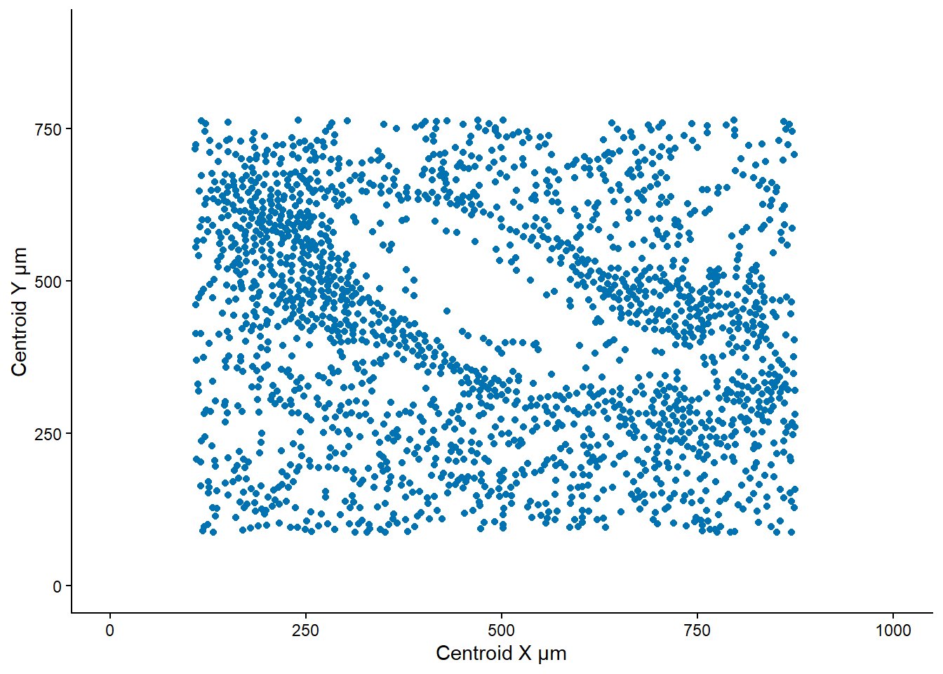
Plot the nuclei as points and add contour lines./绘制细胞核和等高线。
nuclei_contour_plot <- ggplot(df, aes(x = `Centroid X µm`, y = `Centroid Y µm`)) +
  geom_point(color = "#0072B2") + # scatter plot
  geom_density_2d(aes(color = after_stat(level)), bins = 15) + # add contour lines
  scale_color_viridis_c(option = "H") + # set color scale for contour lines
  scale_x_continuous(limits = c(0, 1000)) + # set x limits
  scale_y_continuous(limits = c(0, 900)) + # set y limits
  theme_classic() # apply classic theme

nuclei_contour_plot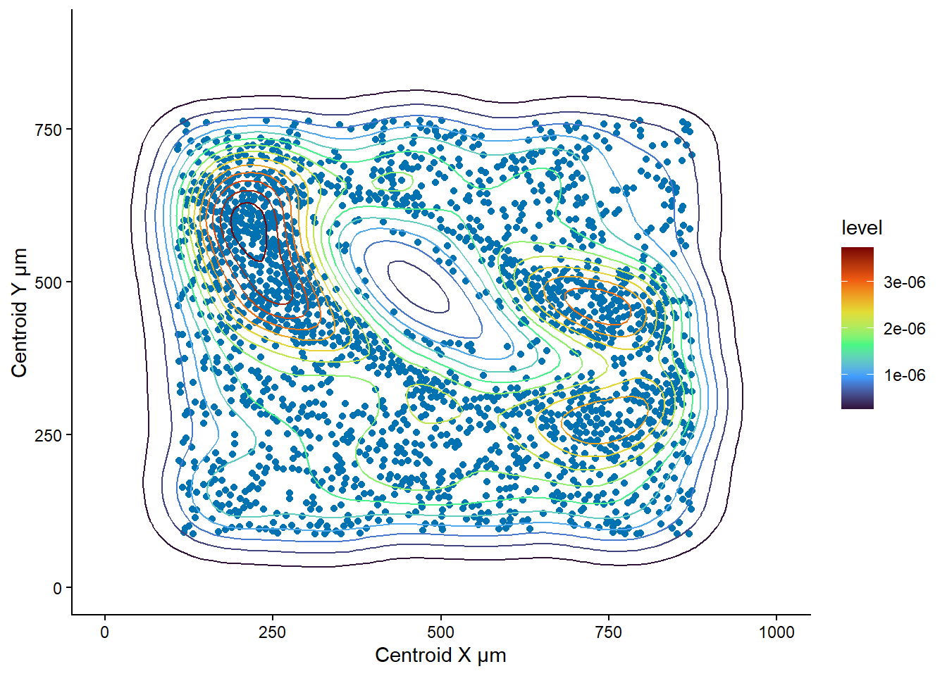
3. Claculate the area of a contour level/计算一个等高线的面积
Extract the data used to create the contour plot/提取用于创建等高线图的数据
plot_data <- nuclei_contour_plot |>
  ggplot_build() |>
  pluck("data", 2) # extract the data used to create the contour plot

plot_data |> dim() # display the dimensions of the contour plot data
[1] 3915 12plot_data |> distinct(level) # display distinct levels in the contour plot level
1 2.666667e-07
2 5.333333e-07
3 8.000000e-07
4 1.066667e-06
5 1.333333e-06
6 1.600000e-06
7 1.866667e-06
8 2.133333e-06
9 2.400000e-06
10 2.666667e-06
11 2.933333e-06
12 3.200000e-06
13 3.466667e-06
14 3.733333e-06Select a level (e.g. 8th level)./选择一个等高线(比如第8个level)
levels <- plot_data |> distinct(level) # select the unique levels
plot_data_8 <- plot_data |>
  filter(level == levels$level[8]) # filter the data for the 8th level
Plot the 8th contour level./绘制第8个等高线
contour_8 <- ggplot(plot_data_8, aes(x = x, y = y, group = group)) +
  geom_polygon(color = "blue", fill = "lightblue", alpha = 0.5) + # draw the polygon with specified fill and border color
  theme_classic() + # apply classic theme
  scale_x_continuous(limits = c(0, 1000)) + # set x limits
  scale_y_continuous(limits = c(0, 900)) # set y limits

contour_8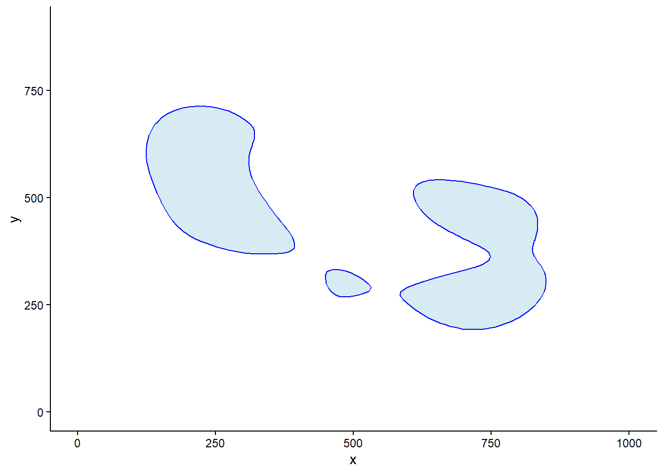
Calculate the area and center of the 8th contour level using the pracma package/计算第8个等高线的面积和中心坐标。
# set a function to calculate the area and center of a polygon
calculate_polygon_area_pracma <- function(df) {
  x <- df$x
  y <- df$y
  n <- length(x)

  area <- polyarea(x, y) # calculate the area
  center <- poly_center(x, y) # calculate the center
  return(c(area, center))
}

# use the function to calculate the area and center of each polygon of 8th contour level
area_each_polygon <- plot_data_8 |>
  group_by(group) |>
  group_map(~ calculate_polygon_area_pracma(.x))

area_each_polygon
[[1]]
[1] 60220.5955 244.9297 538.7649
[[2]]
[1] 58107.1948 730.7534 362.4998
[[3]]
[1] 3757.6480 485.9918 299.8639Plot the area of the 8th contour level with the area annotated./绘制面积图,并标注面积
contour_8_area <- ggplot(plot_data_8, aes(x = x, y = y, group = group)) +
  geom_polygon(color = "blue", fill = "lightblue", alpha = 0.5) + # draw the polygon with specified fill and border color
  theme_classic() + # apply classic theme
  scale_x_continuous(limits = c(0, 1000)) + # set x limits
  scale_y_continuous(limits = c(0, 900)) + # set y limits
  annotate("text", x = area_each_polygon[[1]][2], y = area_each_polygon[[1]][3], label = round(area_each_polygon[[1]][1], 2), size = 5, color = "red") + # add the area and center label
  annotate("text", x = area_each_polygon[[2]][2], y = area_each_polygon[[2]][3], label = round(area_each_polygon[[2]][1], 2), size = 5, color = "red") + # add the area and center label
  annotate("text", x = area_each_polygon[[3]][2], y = area_each_polygon[[3]][3], label = round(area_each_polygon[[3]][1], 2), size = 5, color = "red") # add the area and center label

contour_8_area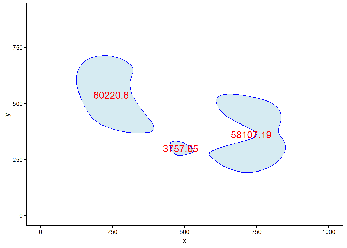
Plot the 8th contour level with the arear annotated on the original image./绘制面积图到原图,并标注面积
ggplot(df, aes(x = `Centroid X µm`, y = `Centroid Y µm`)) +
  geom_polygon(data = plot_data_8, aes(x = x, y = y, group = group), fill = "#cccccc") +
  geom_point(color = "#969696") + # scatter plot
  geom_density_2d(bins = 15, color = "#cbc9e2") + # add contour lines
  scale_x_continuous(limits = c(0, 1000)) + # set x limits
  scale_y_continuous(limits = c(0, 900)) + # set y limits
  theme_classic() + # apply classic theme
  annotate("text", x = area_each_polygon[[1]][2], y = area_each_polygon[[1]][3], label = round(area_each_polygon[[1]][1], 2), size = 6, color = "#f03b20") + # add the area and center label
  annotate("text", x = area_each_polygon[[2]][2], y = area_each_polygon[[2]][3], label = round(area_each_polygon[[2]][1], 2), size = 6, color = "#f03b20") + # add the area and center label
  annotate("text", x = area_each_polygon[[3]][2], y = area_each_polygon[[3]][3], label = round(area_each_polygon[[3]][1], 2), size = 6, color = "#f03b20") # add the area and center label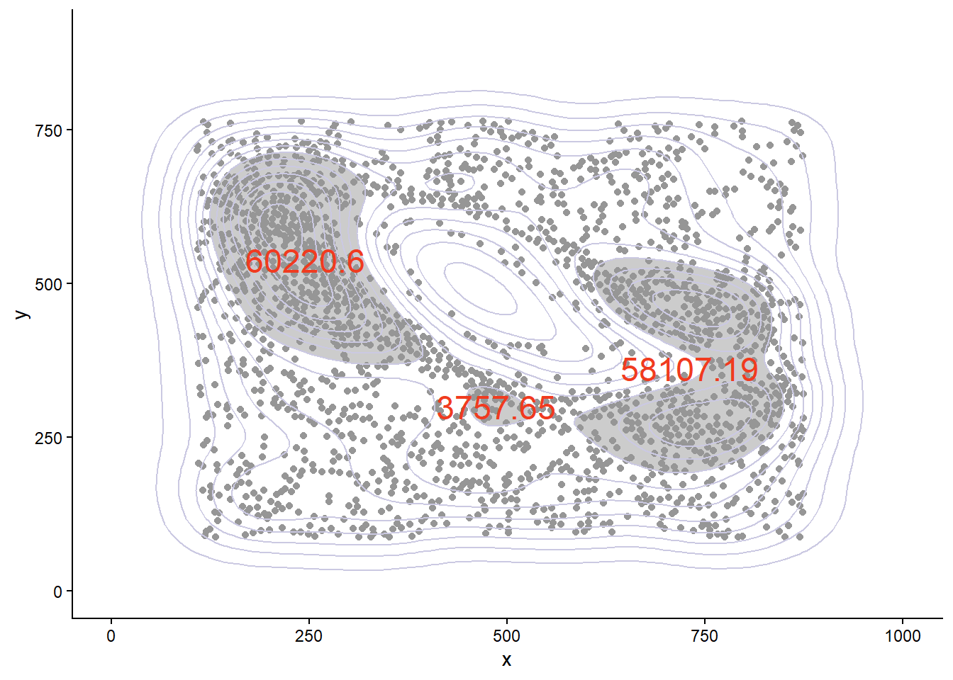
4. “银行系”的起源